
RAG Explained: Understanding Embeddings, Similarity, and Retrieval
Let's take a closer look at how the retrieval mechanism works


In my last posts, I walked through building a simple RAG pipeline using OpenAI’s API, LangChain, and local files, as well as effectively chunking large text files. These posts cover the basics of setting up a RAG pipeline able to generate responses based on the content of local files.
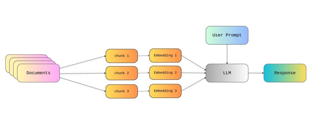
Therefore, so far, we’ve talked about reading the documents from wherever they are stored, splitting them into text chunks, and then creating an embedding for each chunk. After that, we somehow magically pick the embeddings that are appropriate for the user query and generate a relevant response. But it’s important to further understand how the retrieval step of RAG actually works.
Thus, in this post, we’ll take things a step further by taking a closer look at how the retrieval mechanism works and analyzing it in more detail. As in my previous post, I will be using the War and Peace text as an example, licensed as Public Domain and easily accessible through Project Gutenberg.
What about the embeddings?
In order to understand how the retrieval step of the RAG framework works, it is crucial to first understand how text is transformed and represented in embeddings. For LLMs to handle any text, it must be in the form of a vector, and to perform this transformation, we need to utilize an embedding model.
An embedding is a vector representation of data (in our case, text) that captures its semantic meaning. Each word or sentence of the original text is mapped to a high-dimensional vector. Embedding models used to perform this transformation are designed in such a way that similar meanings result in vectors that are close to one another in the vector space. For example, the vectors for the words happy and joyful would be close to one another in the vector space, whereas the vector for the word sad would be far from them.
To create high-quality embeddings that work effectively in an RAG pipeline, one needs to utilize pre-trained embedding models, like OpenAI’s embedding models. There are various types of embeddings one can create and corresponding models available. For instance:
Word Embeddings: In word embeddings, each word has a fixed vector regardless of context. Popular models for creating this type of embedding are Word2Vec and GloVe.
Contextual Embeddings: Contextual embeddings take into account that the meaning of a word can change based on context. Take, for instance, the bank of a river and opening a bank account. Some models that can be used for producing contextual embeddings are BERT and OpenAI’s embedding models (like
text-embedding-ada-002)Sentence Embeddings: These are embeddings capturing the meaning of full sentences. A popular embedding model for creating sentence embeddings is Sentence-BERT.
In any case, text must be transformed into vectors to be usable in computations. These vectors are simply representations of the text. In other words, the vectors and numbers don’t have any inherent meaning on their own. Instead, they are useful because they capture similarities and relationships between words or phrases in a mathematical form.
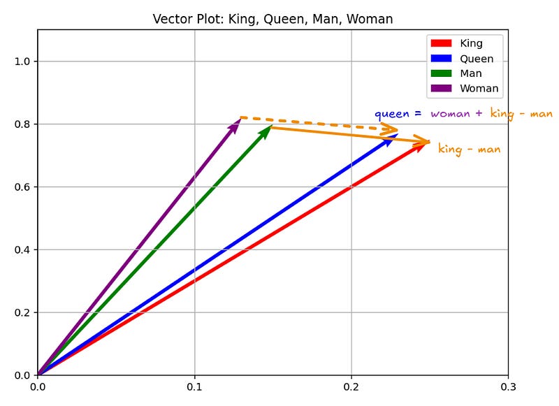
For instance, we could imagine a tiny vocabulary consisting of the words king, queen, woman, and man, and assign each of them an arbitrary vector.
king  = [0.25, 0.75]
queen = [0.23, 0.77]
man   = [0.15, 0.80]
woman = [0.13, 0.82]
Then, we could try to do some vector operations like:
king - man + woman
= [0.25, 0.75] - [0.15, 0.80] + [0.13, 0.82]
= [0.23, 0.77]
≈ queen 👑
Notice how the semantics of the words and the relationships between them are preserved after mapping them into vectors, allowing us to perform operations.
So, an embedding is just that — a mapping of words to vectors, aiming to preserve meaning and relationships between words, and allowing to perform computations with them. We can even visualize these dummy vectors in a vector space to see how related words cluster together.
The difference between these simple vector examples and the real vectors produced by embedding models is that actual embedding models generate vectors with hundreds of dimensions. Two-dimensional vectors are useful for building intuition about how meaning can be mapped into a vector space, but they are far too low-dimensional to capture the complexity of real language and vocabulary. That’s why real embedding models work with much higher dimensions, often in the hundreds or even thousands. For example, Word2Vec produces 300-dimensional vectors, while BERT Base produces 768-dimensional vectors. This higher dimensionality allows embeddings to capture the multiple dimensions of real language, like meaning, usage, syntax, and the context of words and phrases. Ultimately, this two-dimension simplified example allows us to build some intuition on what an embedding is - nonetheless, it is rather simplistic and not necessarily something you should expect to see replicate in real models.
Assessing the similarity of embeddings
After the text is transformed into embeddings, inference becomes vector math. This is exactly what allows us to identify and retrieve relevant documents in the retrieval step of the RAG framework. Once we turn both the user’s query and the knowledge base documents into vectors using an embedding model, we can then compute how similar they are using an appropriate metric like cosine similarity, Euclidean distance (L2 distance), or dot product.
Cosine similarity is a measure of how similar two vectors (embeddings) are. Given two vectors A and B, cosine similarity is calculated as follows:
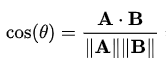
Simply put, cosine similarity is calculated as the cosine of the angle between two vectors, and it ranges from 1 to -1. More specifically:
1 indicates that the vectors are semantically identical (e.g., car and automobile).
0 indicates that the vectors have no semantic relationship (e.g., banana and justice).
-1 indicates that the vectors are perfectly opposite, but in practice, embeddings don’t produce negative similarities, even for antonyms like hot and cold.
This is because even semantically opposite words (like hot and cold) often occur in similar contexts (e.g., it’s getting hot and it’s getting cold). For cosine similarity to reach -1, the words themselves and their contexts would both need to be perfectly opposite—something that doesn’t really happen in natural language. As a result, even opposite words typically have embeddings that are still somewhat close in meaning. In practice, similarity scores are usually positive.
Other similarity metrics apart from cosine similarity include dot product (inner product) and Euclidean distance (L2 distance). Unlike cosine similarity, the dot product and Euclidean distance are magnitude-dependent, meaning that vector length affects the result. To use the dot product as a measure of similarity equivalent to cosine similarity, we must first normalize the vectors to unit length. This is because cosine similarity is mathematically equal to the dot product of two normalized vectors. Thus, similarly to cosine similarity, more similar vectors will have a larger dot product.
On the other hand, Euclidean distance measures the straight-line distance between two vectors in the embedding space. In this case, more similar vectors will have a smaller Euclidean distance.
Back to our RAG pipeline, by calculating the similarity scores between the user’s query embeddings and the knowledge base embeddings, we can identify the chunks of text that are most similar—and therefore contextually relevant—to the user’s question, retrieve them, and then use them to generate the answer.
Finding the top k similar chunks
So, after getting the embeddings of the knowledge base and the embedding(s) for the user query text, this is where the magic happens. What we essentially do is that we calculate the cosine similarity between the user query embedding and the knowledge base embeddings. Thus, for each text chunk of the knowledge base, we get a score between 1 and -1 indicating the chunk’s similarity with the user’s query.
Once we have the similarity scores, we sort them in descending order and select the top k chunks. These top k chunks are then passed into the generation step of the RAG pipeline, allowing it to effectively retrieve relevant information for the user’s query.
To speed up this process, the Approximate Nearest Neighbor (ANN) search is often used. ANN finds vectors that are nearly the most similar, delivering results close to the true top-N but at a much faster rate than exact search methods. Of course, exact search is more accurate; nonetheless, it is also more computationally expensive and may not scale well in real-world applications, especially when dealing with massive datasets.
On top of this, a threshold may be applied to the similarity scores to filter out chunks that do not meet a minimum relevance score. For example, in some cases, a chunk might only be considered if its similarity score exceeds a certain threshold (e.g., cosine similarity > 0.3).
So, who is Anna Pávlovna?
In the ‘War and Peace‘ example, as demonstrated in my previous post, we split the entire text into chunks and then create the respective embeddings for each chunk. Then, when the user submits a query, like ‘Who is Anna Pávlovna?’, we also create the respective embedding(s) for the user’s query text.
import os
from langchain.chat_models import ChatOpenAI
from langchain.document_loaders import TextLoader
from langchain.embeddings import OpenAIEmbeddings
from langchain.vectorstores import FAISS
from langchain.text_splitter import RecursiveCharacterTextSplitter
from langchain.docstore.document import Document

api_key = ‘your_api_key’

# initialize LLM
llm = ChatOpenAI(openai_api_key=api_key, model=”gpt-4o-mini”, temperature=0.3)

# initialize embeddings model
embeddings = OpenAIEmbeddings(openai_api_key=api_key)

# loading documents to be used for RAG
text_folder =  “RAG files”

documents = []
for filename in os.listdir(text_folder):
    if filename.lower().endswith(”.txt”):
        file_path = os.path.join(text_folder, filename)
        loader = TextLoader(file_path)
        documents.extend(loader.load())

splitter = RecursiveCharacterTextSplitter(chunk_size=1000, chunk_overlap=100)
split_docs = []
for doc in documents:
    chunks = splitter.split_text(doc.page_content)
    for chunk in chunks:
        split_docs.append(Document(page_content=chunk))

documents = split_docs

# create vector database w FAISS
vector_store = FAISS.from_documents(documents, embeddings)
retriever = vector_store.as_retriever()

def main():
    print(”Welcome to the RAG Assistant. Type ‘exit’ to quit.\n”)

    while True:
        user_input = input(”You: “).strip()
        if user_input.lower() == “exit”:
            print(”Exiting…”)
            break

        # get relevant documents
        relevant_docs = retriever.invoke(user_input)
        retrieved_context = “\n\n”.join([doc.page_content for doc in relevant_docs])

        # system prompt
        system_prompt = (
            “You are a helpful assistant. “
            “Use ONLY the following knowledge base context to answer the user. “
            “If the answer is not in the context, say you don’t know.\n\n”
            f”Context:\n{retrieved_context}”
        )

        # messages for LLM
        messages = [
            {”role”: “system”, “content”: system_prompt},
            {”role”: “user”, “content”: user_input}
        ]

        # generate response
        response = llm.invoke(messages)
        assistant_message = response.content.strip()
        print(f”\nAssistant: {assistant_message}\n”)

if __name__ == “__main__”:
    main()
In this script, I use LangChain’s retriever object retriever = vector_store.as_retriever(), which by default uses the similarity metric of the underlying FAISS index. FAISS provides two indices:
IndexFlatL2utilizes L2 distance. When using LangChain with FAISS (like we did), the default index is usuallyIndexFlatL2IndexFlatIP, which uses the dot product (inner product)
Therefore, in the initial script, chunks are retrieved using L2 distance as a metric. This script also retrieves by default the k=4 most similar chunks. In other words, what we are doing there is that we retrieve the top k most relevant to the user query chunks based on L2 distance.
Thus, in order to use cosine similarity as the retrieval metric instead of L2, which was in place by default, we need to tweak our initial code a little bit. In particular, we need to normalize the embeddings (both the embeddings of the user’s query and the knowledge base), and configure the vector store to use the dot product (inner product) as the similarity measure instead of L2 distance. In order to normalize the embeddings of the knowledge base, we can add this part after the chunking step:
...

documents = split_docs

# normalize knowledge base embeddings
import numpy as np
def normalize(vectors):
    vectors = np.array(vectors)
    norms = np.linalg.norm(vectors, axis=1, keepdims=True)
    return vectors / norms

doc_texts = [doc.page_content for doc in documents]
doc_embeddings = embeddings.embed_documents(doc_texts)
doc_embeddings = normalize(doc_embeddings)

# faiss index with inner product
import faiss
dimension = doc_embeddings.shape[1]
index = faiss.IndexFlatIP(dimension)  # inner product index
index.add(doc_embeddings)

# create vector database w FAISS
vector_store = FAISS(embedding_function=embeddings, index=index, docstore=None, index_to_docstore_id=None)
vector_store.docstore = {i: doc for i, doc in enumerate(documents)}

retriever = vector_store.as_retriever()

...
Since we are doing everything manually, we can also omit the retriever = vector_store.as_retriever() for now. We also need to add the following part to our main() function, in order to also normalize the user’s query:
 ...

        if user_input.lower() == “exit”:
            print(”Exiting…”)
            break

        # embedding + normalize query
        query_embedding = embeddings.embed_query(user_input)
        query_embedding = normalize([query_embedding])

        # search FAISS index
        D, I = index.search(query_embedding, k=2)

        # get relevant documents
        relevant_docs = [vector_store.docstore[i] for i in I[0]]
        retrieved_context = “\n\n”.join([doc.page_content for doc in relevant_docs])

   ...
Notice how we can explicitly define the number of retrieved chunks k, now set as k=2.
On top of this, in order to print the cosine similarities, I’m going to also add the following part in the main() function:
...
        retrieved_context = “\n\n”.join([doc.page_content for doc in relevant_docs])

        # D contains inner product scores == cosine similarities (since normalized)
        print(”\nTop 5 chunks and their cosine similarity scores:\n”)
        for rank, (idx, score) in enumerate(zip(I[0], D[0]), start=1):
           print(f”Chunk {rank}:”)
           print(f”Cosine similarity: {score:.4f}”)
           print(f”Content:\n{vector_store.docstore[idx].page_content}\n{’-’*40}”)
...
Finally, we can again ask and receive an answer:

... but now we are also able to see the text chunks based on which this answer is created, and the respective cosine similarity scores...
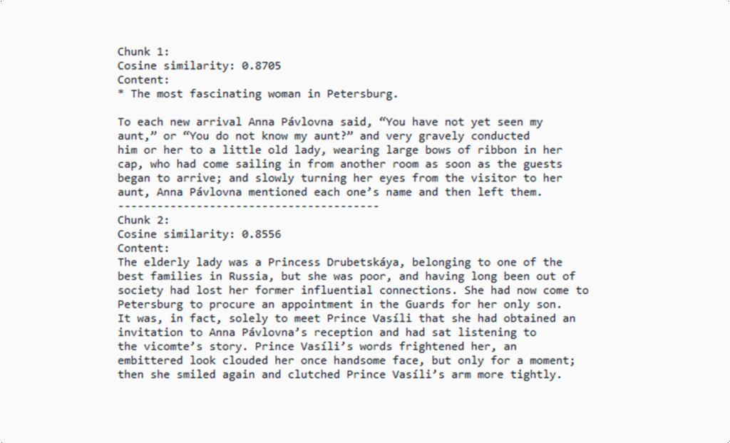
Apparently, different parameters can result in different answers. For instance, we are going to get slightly different answers when retrieving the top k=2, k=4, and k=10 results. Taking into consideration the additional parameters that are used in the chunking step, like chunk size and chunk overlap, it becomes obvious that parameters play a crucial role in getting good results from an RAG pipeline.
Loved this post? Let’s be friends! Join me on 💌 Medium 💼 LinkedIn ☕ Buy me a coffee!
What about pialgorithms?
Looking to bring the power of RAG into your organization?
pialgorithms can do it for you 👉 book a demo today!